 It is well known that daytime winter temperatures on Earth can fall well below -4°F (-20℃ ) in some places, even in midlatitudes, despite warming worries. Sometimes the surface can even drop below -40°F (-40℃ ), which is comparable to the surface of Mars.
What is not so well known is that such cold winter days are colder than they would be with no atmosphere at all! [bold, links added]
How can that be if the atmosphere is like a blanket, according to the standard greenhouse analogy? If the greenhouse analogy fails, what is climate?
Climate computer models from the 1960s could not account for this non-greenhouse-like picture. However, modern computer models are better than those old models, but the climate implications of an atmosphere that cools as well as warms have not been embraced.
Will computer models be able to predict climate after it is? The meteorological program for climate has been underway for more than 40 years. How did it do?
Feynman, Experiment and Climate Models
“Model” is used in a peculiar manner in the climate field. In other fields, models are usually formulated so that they can be found false in the face of evidence. From fundamental physics (the Standard Model) to star formation, a model is meant to be put to the test, no matter how meritorious.
Climate models do not have this character. No observation from Nature can cause them to be replaced by some new form of a model.
Instead, climate models are seen by some as the implementation of perfectly established classical physics expressed on oracular computers, and as such must be regarded as fully understood and beyond falsification. In terms of normal science, this is fantasy.
Modern critics of climate models cite a famous remark of physicist Richard Feynman: “It doesn’t matter how beautiful your theory is, it doesn’t matter how smart you are. If it doesn’t agree with the experiment, it’s wrong.”
Those critics imagine models as theory and observations as experiments. No knowledgeable model builder believes that climate models capture all features of the system well. As such, they disagree with observations.
However, they do not violate Feynman’s edict because climate models are no theory for climate, and observations of an uncontrolled system are no experiment. Feynman was speaking in the context of controlled physical experiments, which cannot be done for the climate.
If a climate model disagrees with data, in principle the sub-grid-scale (more below) of ad hoc climate models can be adjusted to make it agree.
Fortunately, good model builders resist the temptation to overdo such tuning. However, they may do things inadvertently like tune models to be more like each other than like the atmosphere and oceans. [reference 1]
Extreme Computing in Search of Climate
Extreme conditions can compromise any computer calculation, despite popular faith otherwise. Sharp transitions on boundaries, extreme gradients, and extremes in density are examples.
There are also extremes that are often overlooked, e.g., an extreme of time. Direct computation of the meteorological physics for long timescales is extreme in time.
Integrations of classical physics on computers for climatological timescales are unique and unprecedented. Like other forms of extreme computation, there are consequences.
Numerical analysis of computers contends with the finite representation (i.e., a finite number of numbers) of all computers. There are three types of errors that result:
- Round off error: the computer must chop off (truncate) numbers because of space limitations.
- Truncation error: To put an equation onto a computer you must usually chop off (truncate) parts of the physical equations you aim to compute.
- Symmetry Error: How you chop up the equations affects the symmetry (Lie symmetry) of the equations you plan to integrate. This is realized in the violation of conservation laws, which are uniquely important for extreme climate timescales. [reference 2]
The first two on this list are routine numerical analyses that all must face with computer calculations. Mostly they are not a problem, but in serious computing, they come up much more frequently than one might like, and measures must be taken.
The third type of error tells us that the actual computer model equations that take us into the future will usually conserve different things than the original equations. The conservation laws from the original mathematics are broken and replaced with something artifactual.
For example, consider a simple numerical treatment of a pendulum. Typically, such numerical treatments do not conserve energy, even though the original equations do.
For long times the amplitude of the pendulum can grow (unphysically) with time because the energy grows instead of being constant in the numerical system. Note that there are conservation laws, due to symmetries, in dissipative systems, too. [reference 2]
The significance of long-term forecasting is clear. The only tie the present has to the future, through fundamental equations, is in terms of change relative to those properties that are preserved over time.
Change those properties; change the prescribed future. Such change can accrue over long timescales.
Computation for climate regimes has another claim to extremity. The range of spatial scales is extraordinary. There are few other scientific problems that compare.
The finite representation enters here too, inducing something like pixels on a computer screen. Between pixels, nothing is captured. For proper computing, grid spacings must be smaller than anything you hope to capture. All the wiggles in the equation’s solution must be larger than the grid spacing. Everything else is lost.
But the enormous scales and complexity of the climate mean that the wiggles are much smaller than grid spacings. Not even thunderstorms show up given resolutions of 100s of kilometers!
If you put together a grid that could capture all turbulence, say, you’d need a spacing of about 1mm – air’s Kolmogorov cutoff (the smallest turbulent eddy size).
Considering the scale of the Earth, on modern computers, a proper computation of a ten-year forecast for the atmosphere and oceans can be estimated as taking in excess of the age of the Universe, squared.
The climate problem is much too big, and computers remain far too small and slow to do the proper computation for this problem. We can proceed no further unless one compromises to improper computation.
Important processes between the grid points must be treated, but with time-saving, empirically-based replacements for proper physics. These are the sub-grid-scale “parameterizations.”
All climate models are improper in this sense, employing mathematical cartoons instead of the advertised physics. The basis for any unalloyed faith in climate models is thus dispensed with.
Thus, released from the strictures of specific mathematics and physics, models can always be tuned to approximate any observations one wants. If we have future data, we can tune the models to that too. But we cannot adjust for conditions we haven’t encountered yet.
That is a key property of real climate change: conditions that we haven’t encountered yet. So, for climate change, empiricism fails. Only extrapolation remains, making the exercise fundamentally not predictive.
There is yet another issue. Nonlinear equations, distorted into discrete representations on grid points, fed faux physics, integrated for extremely long times, are notoriously computationally unstable.
There has been a long struggle to get these algorithms to settle down and stop wandering off into fantasyland – the gradual loss of system mass, negative densities, and other wonders.
To get these problems under control, models had non-physical energy flows injected into them to keep them stable. These were called flux adjustments in the AR4. They were like reigns for a bronco. [reference 3 – see bottom of this page]
In contrast, modern versions are so stable that nothing happens unless pushed from the outside. Models exhibit no natural variability over long times (white spectra). But instability is also a real-world property.
Are computational stabilization schemes too aggressive, throwing the baby out with the bathwater? Have they encountered computational over-stabilization? [reference 4] Is their long-term stability a bug or a feature?
Some modelers believe the latter. They believe that models have discovered what climate is. Thus, they contend that climate is a “boundary value problem,” as startup conditions no longer matter in the long term.
If true, an observer living on climate timescales would experience no variability – nothing analogous to weather. Every moment would be like the last. Any change would strictly be a matter of external causes.
However, there is no known way to deduce it from first principles, and long-term internal variability is evident. [reference 5 & 5a]
Closure and the Climate Snipe Hunt
Barry Saltzman worked on finding climate from first principles (directly from the fundamental equations), seeking a natural separation between meteorology and climate regimes. [reference 6]
One seeks averaged (climate) equations that are physically consistent with the meteorological regime while also being able to “ignore” it. Fortunately, Nature separates itself from such regimes.
For example, we can ignore quantum mechanics on our trips to the grocery store. Climate would find a coherent definition and meaning in a theory that could “ignore” in this way. This property is called “closure.” It would give otherwise unmoored computer models something to aim for.
But Saltzman and his contemporaries chose a tough path. The closure problem of turbulence was known to be and remains one of the fundamental unsolved problems in science, and climate contains turbulence. One of Saltzman’s efforts along this line led directly to Lorenz’s work, which revolutionized modern science.
While that is quite an accomplishment, he gave up on his agenda, in the end, ultimately deferring to a version of the aforesaid meteorological model program for discovering what climate is. [reference 3 – see bottom of this page]
Meanwhile, ironically extending from Lorenz in part, a small revolution in other fields of science emerged. Ideas like sensitivity to initial conditions, bifurcation, fractals, and complex system dynamics rose in importance. Such ideas have come late to thinking about climate and models, although sensitivity, known as “natural variability,” was already in play.
Few know that climate models cope with this by something called “ensemble averaging.” A single computation of the future can’t address such sensitivity, so the alternative offered is to do the integration repeatedly with a collection (or ensemble) of slightly different initial values.
The average over these is presented as the future. It seems technical, but in terms of the future it is something like the difference between, “You will meet a tall handsome stranger,” and “you may or may not meet an average person.” Forecasts like that are difficult to falsify.
The depth of difficulty of the scientific problem is obscured by the machinery inherited from the radiative-convective-model picture originating in the 60s [reference 7 and 7a], which is peculiarly imposed on modern models.
We imagine in accordance with radiative-convective-model thinking that an integral over a temperature field (temperature index) is proportional to an integral over the radiation field (changes in infrared gas amounts). The constant of proportionality is known as the “climate sensitivity.”
Much effort has gone into determining its “correct” value in the context of climate models. But such a relationship implies that these integrals can be related to each other in a function, which can ignore the underlying meteorology.
That is, it is a claim of closure, and tantamount to a definition of climate. There is no reason to support this claim in Nature. If this function does not exist, neither does climate sensitivity, and the models that conform to this picture are falsified. [reference 8]
A completely different modern approach to climate and climate change is through bifurcation. Bifurcation is a rich subject, existing prior to rudimentary thoughts about “tipping points.” Complex systems can change qualitatively with very small changes of a control parameter for some family of differential equations.
For climate change, one sort of chaos-inflected flow pattern would change to a different one in this picture. Persistent new weather patterns result. This different approach has little to do with temperature. There is practical climate change possible without any “warming” in this picture!
Bifurcation was put directly into the climate context through fluid dynamics on a rotating sphere. [reference 9] Lewis and Langford generated something close to the famous three-cell Hadley circulation spontaneously from first principles!
Moreover, this circulation emerged as a result of a bifurcation process in terms of the equator-pole surface temperature gradient (not temperature!). The bifurcation turned out to be a hysteresis bifurcation (cubic normal form). The familiar Hadley circulation changed into a different circulation (different “climate”) but did not change back when the control parameter was reversed! Irreversible climate change?
Conclusions
A physical definition for climate remains scientifically elusive because it represents a deep problem that neither elegant theories nor brute force computations have succeeded in getting a foothold on. Without that definition, the question posed by the title cannot be answered.
There are many paths yet to explore, but they are buried by the greenhouse mindset inherited from the models of the 1960s. It makes this deep problem seem trivial and it invites the vision of one temperature-controlled solely by infrared active gases.
That is the basis of climate sensitivity, which amounts to a dubious claim of closure for the climate problem. However, this function need not exist in Nature.
This questionable closure invites the vision of climate as a control problem. But it would have control over something that is not actually climate through a function that exists only in the radiative-convective models.
This vision is itself unfalsifiable. Following it ensures that we only fool ourselves, because as Feynman also said, “Nature can’t be fooled.”
Read rest at BigPicNews


The UN IPCC has stated that as climate is a non linear coupled, chaotic system, longer term forecasts are impossible. End of story. No computer can possibly overcome this basic fact, not least because modern physics is not settled and absolute anyway. We do not even know what physis is. Computer models do not include even all known factors, let alone unknown ones.
A computer model is only as honest as the person who create and design them and id that person has political driven then the model is not honest
Admittedly, this article is well ABOVE my scientific “pay grade.” I think the bottom line is the climate is complex and chaotic. Based on “hindcasts” of existing models with creditable (observed) temperature data it would appear that we don’t fully understand all the variables. Given the size & scope of the atmosphere, to think one component (CO2) is the PRIMARY driver of modest warming over the past 150 years seems dubious. Put simply, I think a bit more humility by elements in the scientific community is in order. There is a LOT we don’t yet understand. I think most rational observers would agree. It would appear VERY FOOLISH to wreck our entire (modern) domestic energy system based on models that very well could be completely wrong. My impression is the science is FAR from “settled”…